N-Body Simulation

Start: 10/9/2018
Due: 10/19/2018, by the beginning of class
Collaboration: individual
Important Links: style guidelines, Checklist, nbody.zip, stdlib.jar, gradesheet

This assignment was developed by Robert Sedgewick and Kevin Wayne, Princeton University. Original language was Java.

Goal

Write a program to simulate the motion of n particles in the plane, mutually affected by gravitational forces, and animate the results. Such methods are widely used in cosmology, semiconductors, and fluid dynamics to study complex physical systems. Scientists also apply the same techniques to other pairwise interactions including Coulombic, Biot–Savart, and van der Waals.

Context

In 1687, Isaac Newton formulated the principles governing the motion of two particles under the influence of their mutual gravitational attraction in his famous Principia. However, Newton was unable to solve the problem for three particles. Indeed, in general, solutions to systems of three or more particles must be approximated via numerical simulations.

Program specification

Write a Kotlin program Nbody.kt that

• Takes two Double command-line arguments—the duration of the simulation (Τ) and the simulation time increment (Δt).
• Reads in the details of the universe to be simulated from standard input using java.util.Scanner, using several parallel arrays to store the data.
• Simulates the universe, starting at time t = 0.0, and continuing in Δt increments as long as t < Τ, using the leapfrog scheme described below.
• Animates the results to standard drawing using StdDraw.
• Prints the state of the universe at the end of the simulation (in the same format as the input file) to standard output using println.

Input format

The input format is a text file that contains the information for a particular universe (in SI units).

• The first value is an integer n which represents the number of particles. The second value is a real number radius which represents the radius of the universe; it is used to determine the scaling of the drawing window (which displays particles with x- and y-coordinates between −radius and +radius).
• Next, there are n lines (one for each particle), with each line containing 6 values. The first two values are the x- and y-coordinates of the initial position; the next pair of values are the x- and y-components of the initial velocity; the fifth value is the mass; the last value is a String that is the name of an image file used to display the particle.
• The remainder of the file (optionally) contains a description of the universe, which your program must ignore.

As an example, planets.txt contains real data from part of our Solar System.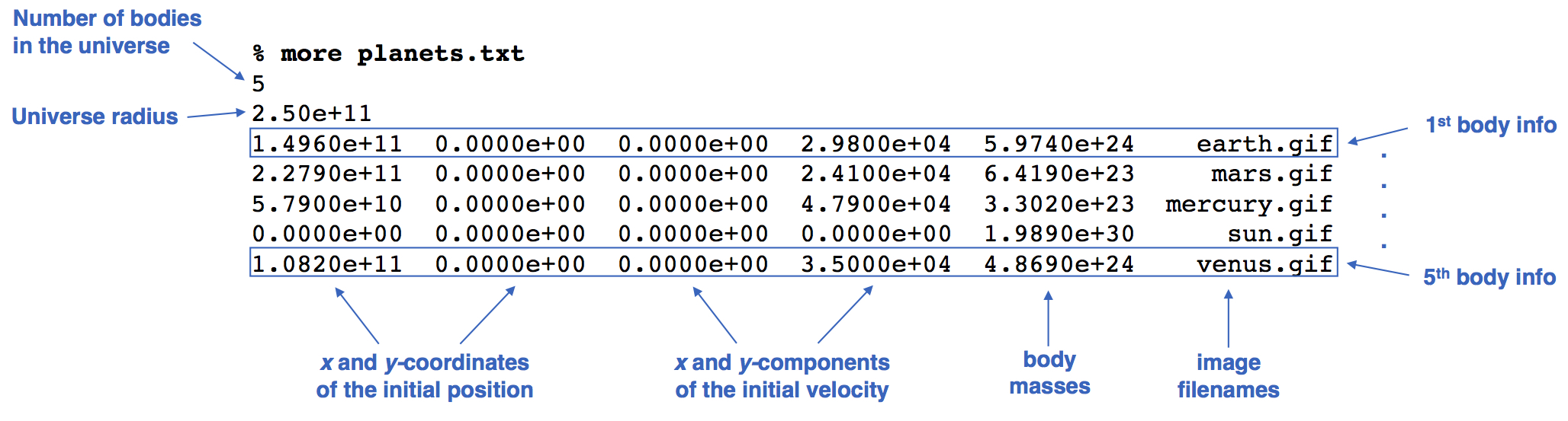

Getting started

Before you begin coding, do the following.

• Get familiar with the command line. Review how to compile and execute a program from the command line.

• Get familiar with Sedgewick’s standard libraries. To use his standard libraries, you need to have stdlib.jar available to your terminal application. We will use these two libraries from stdlib: StdDraw (for drawing results to standard drawing), and StdAudio (for sending sound to standard audio). You can ignore the rest of stuff in stdlib.

• Download the data files. To test your program, you will need planets.txt and the accompanying image and sound files. The zip file nbody.zip contains these files, along with a readme.txt template and additional test universes.

Compiling and executing your program

I’m assuming

1. You have set up your environment variable CLASSPATH to include your current directory and path name to the file stdlib.jar, and also alias kotlinc and kotlin. See CLASSPATH how-to.
2. You have unzipped the provided file nbody.zip into your current directory. See zip how-to.

To compile your program from the command line, type the following in your terminal application (linux terminal, SWL bash, or OS X Terminal):

$ kotlinc Nbody.kt

To execute your program from the command line, and redirecting from the file planets.txt to standard input, type:

$ kotlin NbodyKt 157788000.0 25000.0 < nbody/planets.txt

(I’m assuming throughout the writeup that you have unzipped the given nbody.zip into the directory where you are working on the source code for this project.) After the animation stops, your program must output the final state of the universe in the same format as the input, e.g.:

5
2.50e11
 1.4925e+11 -1.0467e+10  2.0872e+03  2.9723e+04  5.9740e+24    earth.gif
-1.1055e+11 -1.9868e+11  2.1060e+04 -1.1827e+04  6.4190e+23     mars.gif
-1.1708e+10 -5.7384e+10  4.6276e+04 -9.9541e+03  3.3020e+23  mercury.gif
 2.1709e+05  3.0029e+07  4.5087e-02  5.1823e-02  1.9890e+30      sun.gif
 6.9283e+10  8.2658e+10 -2.6894e+04  2.2585e+04  4.8690e+24    venus.gif

Simulating the universe: the physics

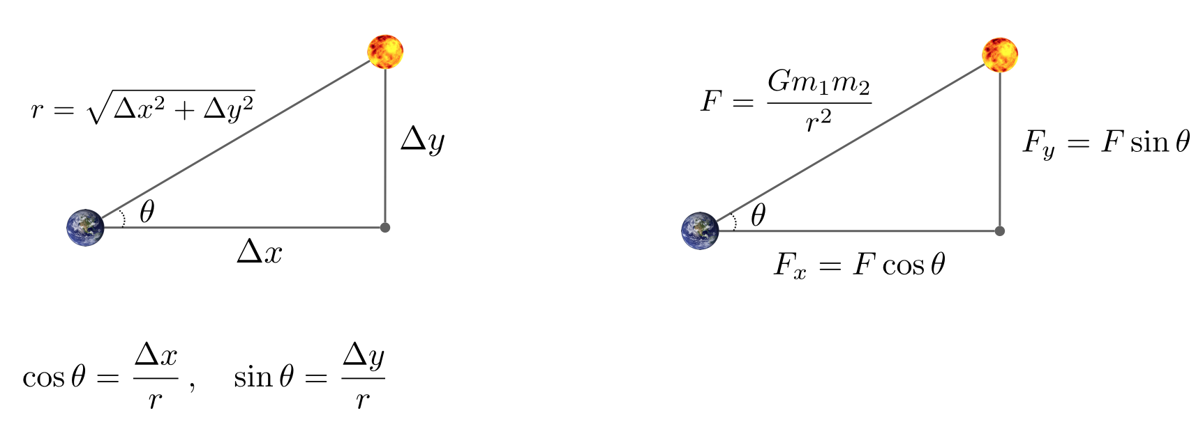
We review the equations governing the motion of the particles, according to Newton's laws of motion and gravitation. Don't worry if your physics is a bit rusty; all of the necessary formulas are included below. We'll assume for now that the position (p_x, p_y) and velocity (v_x, v_y) of each particle is known. In order to model the dynamics of the system, we must know the net force exerted on each particle.

• Pairwise force. Newton's law of universal gravitation asserts that the strength of the gravitational force between two particles is given by the product of their masses divided by the square of the distance between them, scaled by the gravitational constant G (6.67 × 10 ⁻¹¹ N·m ²·kg ⁻²). The pull of one particle towards another acts on the line between them. Since we are using Cartesian coordinates to represent the position of a particle, it is convenient to break up the force into its x- and y-components (F_x, F_y) as illustrated here.
• Net force. The principle of superposition says that the net force acting on a particle in the x- or y-direction is the sum of the pairwise forces acting on the particle in that direction.
• Acceleration. Newton's second law of motion postulates that the accelerations in the x- and y-directions are given by: a_x = F_x / m, a_y = F_y / m.

Simulating the universe: the numerics

We use the leapfrog finite difference approximation scheme to numerically integrate the above equations: this is the basis for most astrophysical simulations of gravitational systems. In the leapfrog scheme, we discretize time, and update the time variable t in increments of the time quantum Δt (measured in seconds). We maintain the position (p_x, p_y) and velocity (v_x, v_y) of each particle at each time step. The steps below illustrate how to evolve the positions and velocities of the particles.

• Step A (calculate the forces). For each particle, calculate the net force (F_x, F_y) at the current time t acting on that particle using Newton's law of gravitation and the principle of superposition. Note that force is a vector (i.e., it has direction). In particular, Δx and Δy are signed (positive or negative). In the diagram above, when you compute the force the sun exerts on the earth, the sun is pulling the earth up (Δy positive) and to the right (Δx positive).
• Step B (update the velocities and positions). For each particle:

1. Calculate its acceleration (a_x, a_y) at time t using the net force computed in Step A and Newton's second law of motion: a_x = F_x / m, a_y = F_y / m.
2. Calculate its new velocity (v_x, v_y) at the next time step by using the acceleration computed in (i) and the velocity from the old time step: Assuming the acceleration remains constant in this interval, the new velocity is (v_x + Δt a_x, v_y + Δt a_y).
3. Calculate its new position (p_x, p_y) at time t + Δt by using the velocity computed in (ii) and its old position at time t: Assuming the velocity remains constant in this interval, the new position is (p_x + Δt v_x, p_y + Δt v_y).

• Step C (draw the universe).  Draw each particle, using the position computed in Step B.

Do not interleave steps A and B(iii); otherwise, you will be computing the forces at time t using the positions of some of the particles at time t and others at time t + Δt. The simulation is more accurate when Δt is very small, but this comes at the price of more computation.

Creating an animation

Draw each particle at its current position to standard drawing, and repeat this process at each time step until the designated stopping time. By displaying this sequence of snapshots (or frames) in rapid succession, you will create the illusion of movement. After each time step, draw the background image starfield.jpg; redraw all the particles in their new positions; and control the animation speed (about 40 frames per second looks good).

You will call several methods from the StdDraw library.

Optional finishing touch

For a finishing touch, play the theme to 2001: A Space Odyssey using the StdAudio library and the audio file 2001.wav. It's a one-liner using the method StdAudio.play().

Challenge for the bored

There are limitless opportunities for additional excitement and discovery here. Create an alternate universe (using the same input format). Try adding other features, such as supporting elastic or inelastic collisions. Or, make the simulation three-dimensional by doing calculations for x-, y-, and z-coordinates, then using the z-coordinate to vary the sizes of the planets. Add a rocket ship that launches from one planet and has to land on another. Allow the rocket ship to exert force with the consumption of fuel.

Gradesheet

We will use this gradesheet when grading your work.

Submission

Zip up your Nbody.kt and the completed readme.txt files and submit via Moodle. See zip how-to for how to zip up files.