Simulations

Flipping a Fair Coin

You can simulate flipping a fair coin by running the command below. You get one of two possible outcomes, either a Head or a Tale.

sample( x=c("Head", "Tail"), size=1, replace=TRUE);

## [1] "Head"

You can simulate multiple coin flips by changing the size=1 statement. Here you will simulate 25 coin tosses.

sample( x=c("Head", "Tail"), size=25, replace=TRUE);

##  [1] "Head" "Tail" "Tail" "Tail" "Tail" "Tail" "Tail" "Tail" "Tail" "Tail" "Head" "Head" "Tail"
## [14] "Head" "Tail" "Tail" "Tail" "Head" "Tail" "Head" "Head" "Tail" "Tail" "Tail" "Head"

You can save the results of your experiment by assigning it to a variable. By adding my.sample = at the beginning of the line the output is saved to a variable so you can look at it later. You can look at the results by typing my.sample. You can also look at the results in a frequency table or bar chart.

Create the Data

my.sample <- sample( x=c("Head", "Tail"), size=25, replace=TRUE); # creates the variable

Display the Data

my.sample; # Displays the output

##  [1] "Head" "Tail" "Head" "Tail" "Head" "Tail" "Head" "Head" "Tail" "Head" "Tail" "Tail" "Tail"
## [14] "Head" "Tail" "Tail" "Head" "Head" "Head" "Head" "Head" "Head" "Head" "Tail" "Head"

Frequency Table

table(my.sample);

## my.sample
## Head Tail 
##   15   10

Bar Plot

barplot(table(my.sample)/length(my.sample), ylab="Percent", xlab="Outcome", main="Distribution for Flipping a Fair Coin", col="yellow");  # Plots the data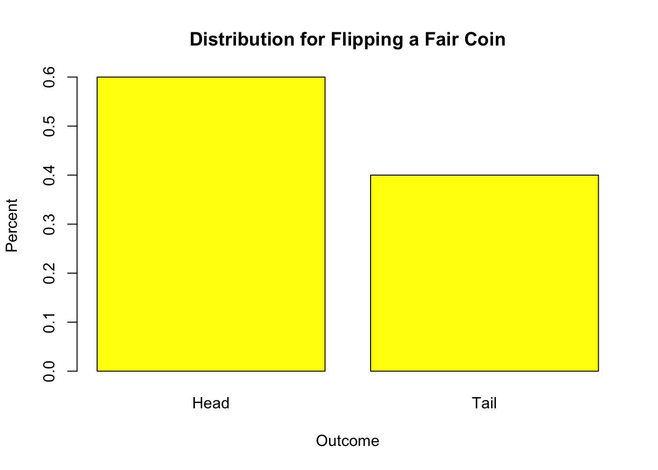

Rolling a Fair Die

By typing the commands below you can simulate rolling a six-sided fair die. You can save the results to a variable or take multiple samples by modifying the code.

die <- c(1,2,3,4,5,6);  # creates the variable
sample(x=die, size=1, replace=TRUE);  # samples 1 roll of the di

## [1] 6

Loaded Die and Unfair Coins

By adding the phrase prob = to the sample statement you can change the probability distribution from the default, uniform distribution, to any distribution you wish. Here it is set so that a Head is flipped with a probability of .75 and Tail is flipped with a probability of .25.

sample( x=c("Head", "Tail"), prob=c(.75, .25), size=25, replace=TRUE);

##  [1] "Head" "Head" "Head" "Head" "Head" "Head" "Head" "Head" "Head" "Head" "Tail" "Head" "Head"
## [14] "Head" "Tail" "Head" "Head" "Head" "Head" "Head" "Tail" "Head" "Head" "Head" "Head"

Rolling Multiple Fair Die

You can simulate many coins and dice simultaneously. Simulations like this may help you address questions that ask what is the distribution of Y where Y = X1 + X2.

Die 1

die1 <- sample(x=c(1,2,3,4,5,6), size=500, replace=TRUE);  

table(die1); 

## die1
##  1  2  3  4  5  6 
## 69 98 65 93 79 96

barplot(table(die1)/length(die1), ylab="Percent", xlab="Outcome", main="Distribution of the First Die", ylim=c(0,.2), col="red");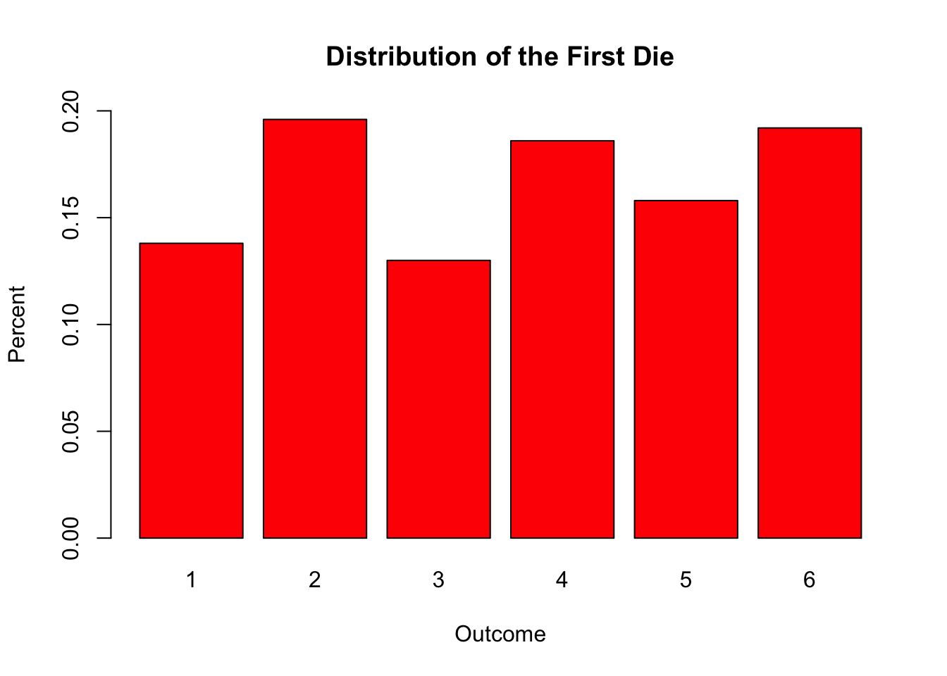 

Die 2

die2 <- sample(x=c(1,2,3,4,5,6), size=500, replace=TRUE);  

table(die2); 

## die2
##  1  2  3  4  5  6 
## 87 90 77 75 78 93

barplot(table(die2)/length(die2), ylab="Percent", xlab="Outcome", main="Distribution of the Second Die", ylim=c(0,.2), col="blue");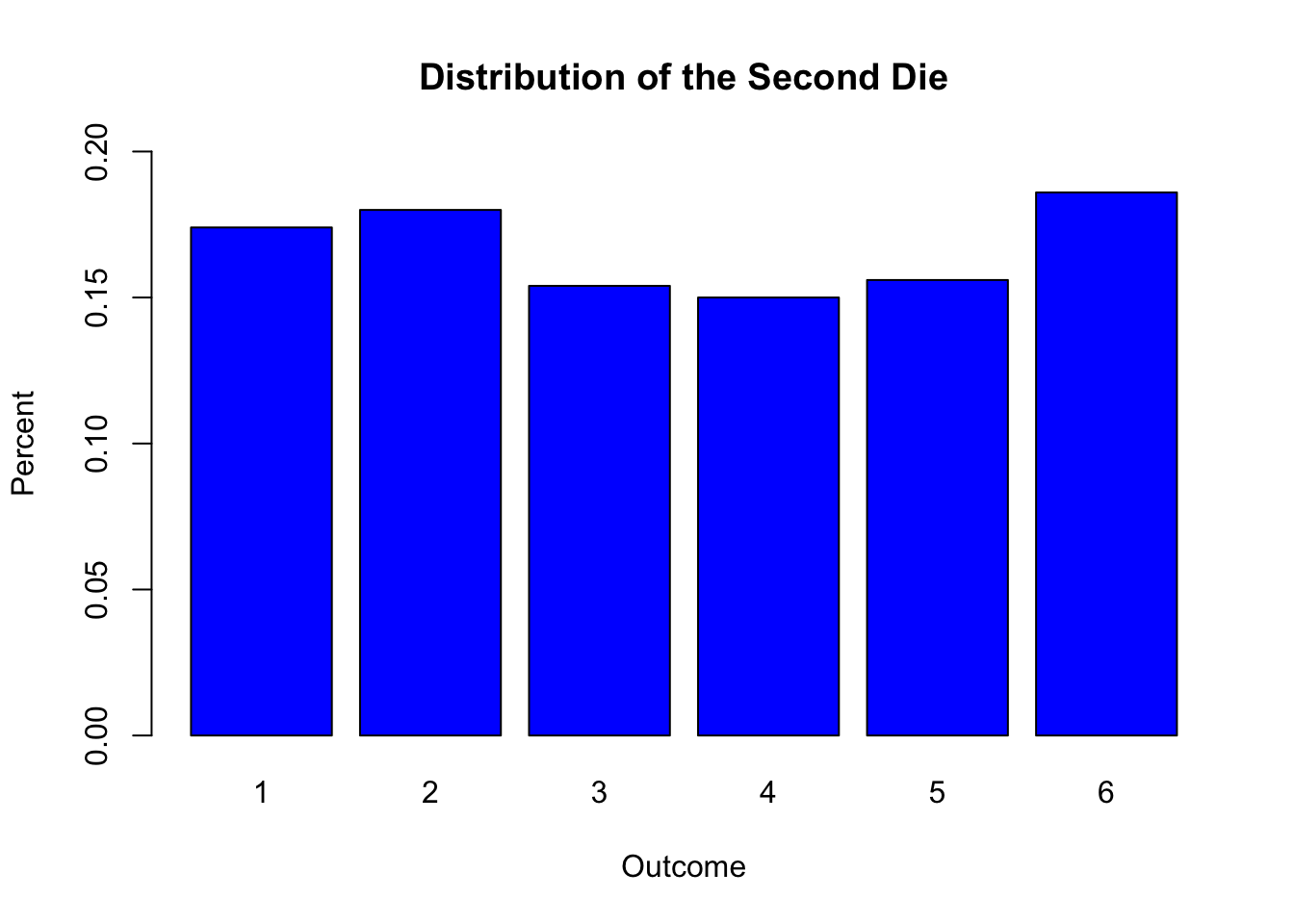 

Die 1 + Die 2

table(die1+die2); 

## 
##  2  3  4  5  6  7  8  9 10 11 12 
## 12 27 41 63 58 85 58 61 49 33 13

barplot(table(die1+die2)/length(die2), ylab="Percent", xlab="Outcome", main="Distribution of the Dice Sum", ylim=c(0,.2), col="purple");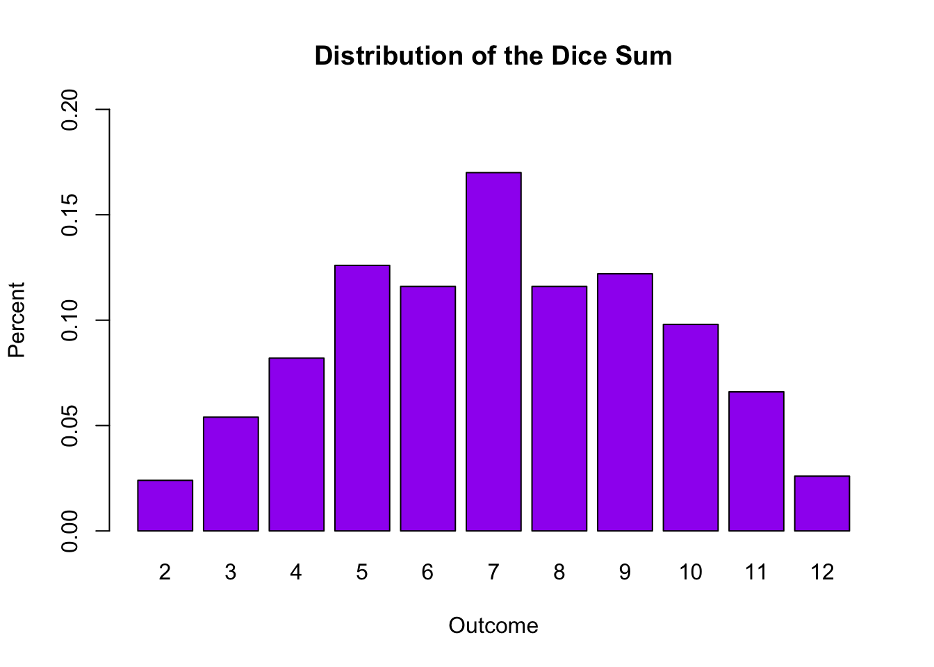 

Mathematicss, Computer Science, and Statistics Department Gustavus Adolphus College