The software used in this course is called R Studio. R Studio is free and exists as a downloadable application as well as a web based application. R Studio is installed on the computers in the MCS department and is available on the Gustavus Virtual Lab. You can learn more about, and download, R Studio here. Gustavus hosts its own web based version of R Studio which can be found at rstudio.gac.edu.

There are many websites designed to provide help on how to use R, R Studio, and R Markdown. Here are some of the more popular websites:

R Studio on the Web

After going to rstudio.gac.edu you should see a screen that looks like the one below. You can log in with your Gustavus username and password.

Once you login

Once you log in to R Studio you should see a screen that looks like the following.

R Studio uses R and Markdown to generate complicated documents with relatively little overhead. We will be using it to generate statistics, plots, and charts.

Creating a Markdown Document

To create an R markdown file click on File , New File, R Markdown. Give your document a title and click OK. You will be given a document that looks like the one below.

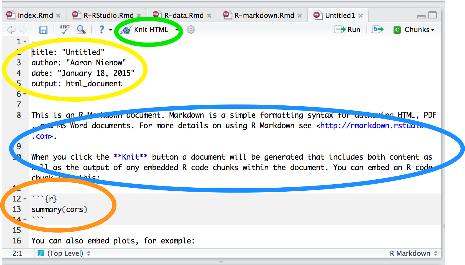
  • The Knit HTML button, (in green), is the button used to generate your document once you are ready.

  • The information in yellow is the information used to generate the HTML document. You will most likely want to change the author option to your name and give your document a better title than "untitled".

  • The text in the blue circle is just text. You can type summaries and comments in the document without having to do anything special. If you look at the provided text you will see that there is a URL included in the text. Markdown provides formatting short-cuts to include links, images, and text formats. For a quick list of these formatting options you can look at the Markdown Basics website.

  • The portion circled in orange is a code chunk. Code chunks produce statistical output. The output is placed right in the document so there is no need to copy and paste. The circled code chunk produces summary statistics for the cars dataset.

Try It

Create a new R Markdown document by clicking on File, New File, R Markdown. You will be prompted to name your document. You can name it whatever you wish. Press the OK button to proceed. Take a look at the R Markdown document that is displayed. The document contains both text and code. Click on the knit HTML button to generate an html document. Notice that the generated document contains text and a scatter plot. Find the code chunk in the markdown document that creates the plot.

Loading Data

There are many ways to load data into R Studio. You can read data directly from a file or you can load data from a URL.

Loading Data from a Package

Fortunately, the authors of "Statistics, Unlocking the Power of Data" also created a package that contains all the datasets mentioned in the book. This package is installed on the Gustavus RStudio server. You need to load the package into your document before you can use it.

library(Lock5Data) # Loads the package.  

Once the package is loaded you should have access to all of the datasets from the package. So, for instance, if the book refers to the AllCountries dataset, you should be able to look up all of the variables in the dataset by typing library(Lock5Data) and ?AllCountries into the console to get a more detailed description of the cases and variables contained in the dataset.

Loading Data from a URL

Two statements are needed to read in data from a web URL.

  • The first gives the web page where the data is stored.

  • The second reads in the data and gives a name to the dataset.

web.url = "www.the.web.address.csv" # The web url
data.name = read.csv(web.url, sep=",", header=TRUE) # reads in the data and gives it a name

To read in and view the data from the example dataset copy the following code and paste it into either the console and press Enter, or into an R Markdown code chunk in a Markdown document and press the knit HTML button.

example.url = "http://homepages.gac.edu/~anienow2/MCS_142/R/example.csv" # web url 
example.data = read.csv(file=example.url, header=TRUE, sep=",") # dataset name 
example.data  # Displays the data

Loading Data from a File

Loading data can be done by clicking on the Environment tab in the upper right window of R Studio. Then click on Import Dataset and choose From Text File.

If you are loading data from a file make sure the file is saved as a .csv file, (.csv stands for comma separated variable). If the file is not a .csv file you can make one by opening the file in Excel or Numbers by using the Save As option in the File menu.

After you have selected the file, you will be presented with the following screen. Be sure to give the data a meaningful name. Besides naming the dataset you should not have to change any of the options on this screen. Once you load the data it will be displayed in the upper left window.

Once you have loaded the data, either from a URL or from a file, you should see a line of code in the console, bottom left window, that looks similar to the code below. This code was generated when the file was loaded.

the.data <- read.csv("http://homepages.gac.edu/~anienow2/MCS_142/R/example.csv", header=TRUE, sep=",")
View(the.data)

Try It

Either read the data from http://homepages.gac.edu/~anienow2/MCS_142/R/example.csv or save the file and read it in. You do not need to do both. The data from the file should look like the following.

##     Name Height Eye.Color   Hand Gender
## 1 Shelly     55      Blue  Right      F
## 2  Alvin     60     Green   Left      M
## 3  Simon     67      Blue  Right      M
## 4   Theo     72     Green  Right      M
## 5  Nicki     54     Brown  Right      F

Saving a Document

Once you have your document ready to turn in you need to save it. By default your R Markdown document and your output document are saved on the RStudio server. If you would like a copy saved to your computer you need to click on the File tab, circled in green, at the top of the output document. Next you need to select the file you wish to save. Do this by checking the box next to the file you want, circled in blue. Finally, click on the More button, circled in yellow. There you should see the option to Export your selection. Select Export and download the document to your computer.

Once you have exported the document to your computer you may want to open the document to make sure that is saved correctly.

Mathematicss, Computer Science, and Statistics Department Gustavus Adolphus College